PyTorch Tutorial
Simple usage example
import torch
import utils
import dataloader
from gnn_wrapper import GNNWrapper, SemiSupGNNWrapper

# define GNN configuration
cfg = GNNWrapper.Config()
cfg.use_cuda = use_cuda
cfg.device = device

cfg.activation = nn.Tanh()
cfg.state_transition_hidden_dims = [5,]
cfg.output_function_hidden_dims = [5]
cfg.state_dim = 2
cfg.max_iterations = 50
cfg.convergence_threshold = 0.01
cfg.graph_based = False
cfg.task_type = "semisupervised"
cfg.lrw = 0.001

model = SemiSupGNNWrapper(cfg)
# Provide your own functions to generate input data
E, N, targets, mask_train, mask_test = dataloader.old_load_karate()
dset = dataloader.from_EN_to_GNN(E, N, targets, aggregation_type="sum", sparse_matrix=True)  # generate the dataset

model(dset)  # dataset initalization into the GNN

#Training

for epoch in range(args.epochs):
    model.train_step(epoch)
Simple toy example for input formatting
Input composed by two graphs:
This graphs can be described in the EN Input format.
The E matrix describing the first graph ( [[id_p, id_c, graph_id],...]):
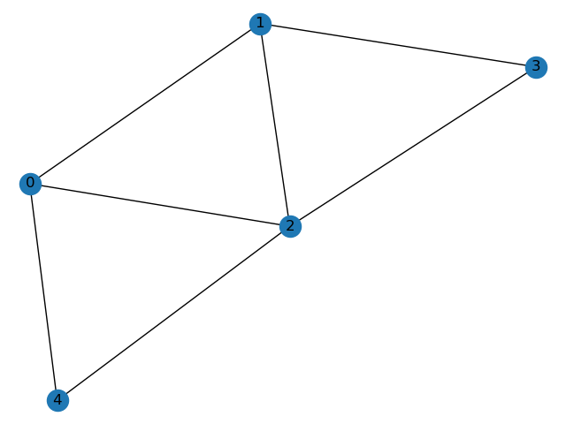
>>> E = [[0 1 0]
         [0 2 0]
         [0 4 0]
         [1 0 0]
         [1 2 0]
         [1 3 0]
         [2 0 0]
         [2 1 0]
         [2 3 0]
         [2 4 0]
         [3 1 0]
         [3 2 0]
         [4 0 0]
         [4 2 0]]
Note the last column, denoting the id (0) of the graph to which the arc belongs.
The E matrix describing the second graph:
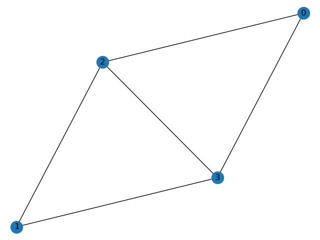
>>> E = [[0 2 1]
         [0 3 1]
         [1 2 1]
         [1 3 1]
         [2 3 1]
         [2 0 1]
         [3 0 1]
         [2 1 1]
         [3 1 1]
         [3 2 1]]
Note the last column, denoting the id (1) of the graph to which the arc belongs .
The global E_tot matrix (with incremental node ids):
>>> E_tot = [[0 1 0]
             [0 2 0]
             [0 4 0]
             [1 0 0]
             [1 2 0]
             [1 3 0]
             [2 0 0]
             [2 1 0]
             [2 3 0]
             [2 4 0]
             [3 1 0]
             [3 2 0]
             [4 0 0]
             [4 2 0]
             [5 7 1]
             [5 8 1]
             [6 7 1]
             [6 8 1]
             [7 5 1]
             [7 6 1]
             [7 8 1]
             [8 5 1]
             [8 6 1]
             [8 7 1]]
The global N matrix ( in this simple case, each node has a different one-hot feature) ([[node_features, graph_id],... ]) :
>>> N = [[1. 0. 0. 0. 0. 0. 0. 0. 0. 0.]
         [0. 1. 0. 0. 0. 0. 0. 0. 0. 0.]
         [0. 0. 1. 0. 0. 0. 0. 0. 0. 0.]
         [0. 0. 0. 1. 0. 0. 0. 0. 0. 0.]
         [0. 0. 0. 0. 1. 0. 0. 0. 0. 0.]
         [0. 0. 0. 0. 0. 1. 0. 0. 0. 0.]
         [0. 0. 0. 0. 0. 0. 1. 0. 0. 0.]
         [0. 0. 0. 0. 0. 0. 0. 1. 0. 0.]
         [0. 0. 0. 0. 0. 0. 0. 0. 1. 0.]]
The from_EN_to_GNN() util takes care of formatting the inputs:
# random labels
labels = np.random.randint(2, size=(N_tot.shape[0]))


# set input and output dim, the maximum number of iterations, the number of epochs and the optimizer
cfg = GNNWrapper.Config()
cfg.use_cuda = True
cfg.device = utils.prepare_device(n_gpu_use=1, gpu_id=0)
cfg.tensorboard = False
cfg.epochs = 500

cfg.activation = nn.Tanh()
cfg.state_transition_hidden_dims = [5,] # hidden dims of the state transition function
cfg.output_function_hidden_dims = [5] # hidden dims of the output function
cfg.state_dim = 5
cfg.max_iterations = 50
cfg.convergence_threshold = 0.01
cfg.graph_based = False
cfg.log_interval = 10
cfg.task_type = "multiclass"
cfg.lrw = 0.001

# model creation
model = GNNWrapper(cfg)
# dataset creation
dset = dataloader.from_EN_to_GNN(E, N_tot, targets=labels, aggregation_type="sum", sparse_matrix=True)  # generate the dataset

model(dset)  # dataset initalization into the GNN
#Training

for epoch in range(1, cfg.epochs + 1):
    model.train_step(epoch)
    if epoch % 10 == 0:
        model.test_step(epoch)
Description
This guide is an introduction to the PyTorch GNN package.
The implementation consists of several modules:
pygnn.py contains the main core of the GNN
gnn_wrapper.py a wrapper (for supervised and semisupervised tasks) handling the GNN
net.py contains the implementation of several state and output networks
dataloader.py contains the data input handling and utils - EN input format utilities, DGL examples
Model definition
Input data
As described in Matrix-based implementation, the computations are based on the arcs in the input graphs. Hence, inputs to the model must be specified as an ordered edge list.
In particular, for each edge, this structure (inp) must contain:
the id of the child node (used to gather its state)
the father and child node labels
the edge label (if available)

Note
We provide a novel utility to compose this kind of input, given a description of the graph dataset in an E-N format. See section EN Input.
ArcNode
In order to aggregate the state per node, a matrix multiplication with an edge–node matrix is performed. The matrix encodes which arcs affect a certain node (see Matrix-based implementation).
This matrix (arcnode) is sparse, to save memory.

EN Input
To simplify the input creation, we provide an utility in the utils.py file, the from_EN_to_GNN(E, N) function.
The user can describe the dataset in the EN format:
- E
numpy array of edges : [[id_p, id_c, graph_id],…]. One row for each arc in the dataset. First column must contain the ids of father nodes, the second column ids of child nodes. The third column contains an id that identifies the graph (to which the node belongs) in the dataset.
- N
numpy array of nodes features - [[node_features, graph_id],… ]. One row for each and every node. A set of columns containing the nodes features. The last column is an id that identifies the graph (to which the node belongs) in the dataset.
The from_EN_to_GNN util takes this two array as input (E N ) and returns the formatted input for the GNN model, inp, arcnode, graphnode.
See Simple toy example for input formatting for a practical example.
State and output function definition
It is possible to define the structure of these functions using the configurator:
>>> cfg.state_transition_hidden_dims = [5, 2]
>>> cfg.output_function_hidden_dims = [5, 3]
>>> cfg.activation = nn.Tanh()
The state dimension, convergence threshold and maximum number of iterations are defined via:
>>> cfg.state_dim = 5
>>> cfg.max_iterations = 50
>>> cfg.convergence_threshold = 0.01
Afterwards, the GNN model can be defined using:
>>> model = GNNWrapper(cfg)
In this way, the model building is complete.
The dataset is generated and given as input to the GNN via:
>>> dset = dataloader.from_EN_to_GNN(E, N_tot, targets=labels, aggregation_type="sum", sparse_matrix=True)  # generate the dataset
>>> model(dset)  # dataset initalization into the GNN
The GNN model handles the dataset. To have more control on the data, check the script gnn_wrapper.py.
Note
In case of a graph-based task, you can specify it trough the config:
>>> cfg.graph_based = True
Training
The Train method runs one epoch of the training procedure:
>>> model.train_step(epoch)
It returns the loss value loss and the number of iteration of the current step convergence procedure it.
Validation
The valid_step method performs the validation (i.e., using the validation set already available in the data) of the model:
>>> model.valid_step(epoch)
Test
The test_step method performs the test phase (i.e., using the test set already available in the data) of the model:
>>> model.test_step(epoch)